R Machine Learning Project - Heart disease Diagnosis
Introduction
With machine learning, And a simple dataset of the patient’s information, We could accurately detect whether is he diagnosed with heart disease or not.
The dataset
Using Cleveland Clinic Foundation dataset (The processed Version), Which contains 14 types of data for each of the 302 patients.
- age
- sex
- cp : chest pain type
- Value 1: typical angina
- Value 2: atypical angina
- Value 3: non-anginal pain
- Value 4: asymptomatic
- trestbps : resting blood pressure (in mm Hg on admission to hospital)
- chol : serum cholestoral in mg/dl
- fbs : (fasting blood sugar > 120 mg/dl)
- 1 = true
- 0 = false
- restecg : resting electrocardiographic results
- Value 0: normal
- Value 1: having ST-T wave abnormality (T wave inversions and/or ST elevation or depression of > 0.05 mV)
- Value 2: showing probable or definite left ventricular hypertrophy by Estes’ criteria
- thalach : duration of exercise test in minutes
- exang : exercise induced angina
- 1 = yes
- 0 = no
- oldpeak : ST depression induced by exercise relative to rest
- slope : the slope of the peak exercise ST segment
- Value 1: upsloping
- Value 2: flat
- Value 3: downsloping
- ca : number of major vessels (0-3) colored by flourosopy
- thal
- 3 = normal
- 6 = fixed defect
- 7 = reversable defect
- num : diagnosis of heart disease (angiographic disease status)
- Value 0: absent
- Value 1-4: present
Data preprocessing
- Loading the data
#specifing the path of the csv file path <- file.path("~","path","to","processed.cleveland.data") #retrieving dataset from csv file data <- read.csv(path,stringsAsFactors = FALSE)- Output screenshot
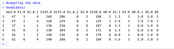
- Output screenshot
- Adding columns names (Not essential)
#data names vector headerNames <- c("age","sex","cp","trestbps","chol","fbs","restecg","thalach","exang","oldpeak","slope","ca","thal","Class") #renaming the dataframe columns colnames(data) <- headerNames- Output screenshot
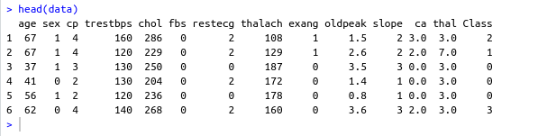
- Output screenshot
- Maping the class column values to binary values : ‘Positive’ & ‘Negative’
#Factoring won't work with binary nums. #So , we used "Postive" , "Negative" names(data) target <- data$Class makeBinary <- function(x){ if(x == 0){ return ("Negative") } else{ return ("Postive") } } target<-sapply(target,makeBinary) data<-cbind(data,target) #adding new col 'target' to data and removing 'class' keep <- c(names(data)[1:13],names(data[15])) data <- data[keep]- Output screenshot
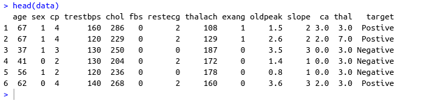
- Output screenshot
- Mutating ‘ca’ & ‘thal’ data-type to numeric and ‘target’ to factor
library(dplyr) data <- data %>% mutate( ca = as.numeric(ca), thal = as.numeric(thal), target = as.factor(target) )- Output screenshot
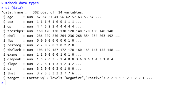
- Output screenshot
- Checking NA values and removing them
sum(is.na(data)) #removing NAs generated by mutate data <- na.omit(data)- Output screenshot
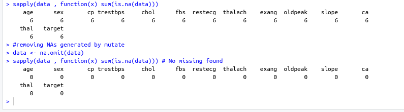
- Output screenshot
Training using caret
library(caret)
cntrl <- trainControl(
    method ="repeatedcv",
    repeats = 5,
    classProbs = TRUE ,
    summaryFunction = twoClassSummary
)
- Naïve Bayes model
set.seed(420) NB_Fit <- train( target ~., data = data, method = "naive_bayes", preProc = c("center","scale"), tuneGrid = expand.grid(.laplace = 0, .usekernel = TRUE, .adjust = 1), trControl = cntrl, metric = "ROC" )- Output screenshot
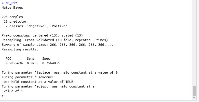
- Output screenshot
- Decision tree model
DT_Fit <- train( target ~., data = data, method = "rpart", preProc = c("center","scale"), tuneLength =15, trControl = cntrl, metric = "ROC" )- Output screenshot
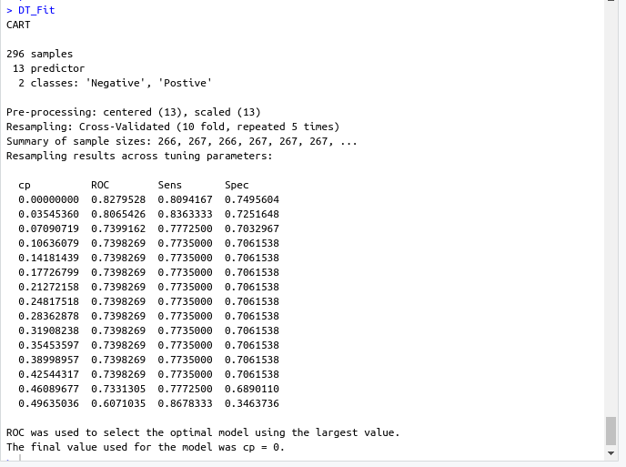
- Output screenshot
- Logistic Regression model
Log_Fit <- train( target ~., data = data, method = "glm", preProc = c("center","scale"), tuneLength =15, trControl = cntrl, metric = "ROC" )- Output screenshot
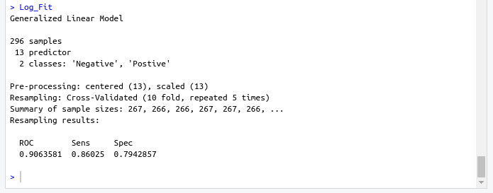
- Output screenshot
models Summary
- Naïve Bayes model
- ROC : 0.9055636
- Sens : 0.8755
- Spec : 0.7564835
- Decision tree model
- ROC : 0.8279528
- Sens : 0.8094167
- Spec : 0.7495604
- Logistic Regression model
- ROC : 0.9063581
- Sens : 0.86025
- Spec : 0.7942857