Heart disease Diagnosis

name: inverse
layout: true
class: center, middle ,inverse
---
# R - Machine Learning Project - Heart disease Diagnosis

.footnote[Go directly to [project site](https://github.com/sbme-tutorials/sbe304-fall19-project-sbe304-2021-team09)]
---

# Introduction
With machine learning, And a simple [dataset](https://archive.ics.uci.edu/ml/datasets/Heart+Disease) of the patient's information, 
We could accurately detect whether he is diagnosed with heart disease or not.

---
layout: false
# The dataset
Using Cleveland Clinic Foundation dataset ([The processed Version](https://archive.ics.uci.edu/ml/machine-learning-databases/heart-disease/processed.cleveland.data)), Which contains 14 types of data for each of the 302 patients.

.left-column[
- **age**       
- **sex**
- **cp**       
- **trestbps**  
- **chol**      
- **fbs**       
- **restecg**   
]
.right-column[
- **thalach**   
- **exang**  
- **oldpeak**   
- **slope**     
- **ca**        
- **thal** 
- **num**

]
---
#The dataset
- **age**       
- **sex**       
- **cp**  :      chest pain type
    - Value 1: typical angina
    - Value 2: atypical angina
    - Value 3: non-anginal pain
    - Value 4: asymptomatic
- **trestbps**  : resting blood pressure (in mm Hg on admission to hospital)
- **chol**      : serum cholestoral in mg/dl
- **fbs**       : (fasting blood sugar > 120 mg/dl) 
  - 1 = true
  - 0 = false
- **restecg**   : resting electrocardiographic results
    - Value 0: normal
    - Value 1: having ST-T wave abnormality (T wave inversions and/or ST elevation or depression of > 0.05 mV)
    - Value 2: showing probable or definite left ventricular hypertrophy by Estes' criteria
---
#The dataset

- **thalach**   : duration of exercise test in minutes
- **exang**     : exercise induced angina 
    - 1 = yes
    - 0 = no
- **oldpeak**   : ST depression induced by exercise relative to rest
- **slope**     : the slope of the peak exercise ST segment
  - Value 1: upsloping
  - Value 2: flat
  - Value 3: downsloping
- **ca**        : number of major vessels (0-3) colored by flourosopy
- **thal**      
  - 3 = normal
  - 6 = fixed defect
  - 7 = reversable defect
- **num** : diagnosis of heart disease (angiographic disease status)
    - Value 0: absent
    - Value 1-4: present

---
template: inverse
# Data preprocessing
---

# Data preprocessing

.left-column[
  ###1. Loading the data
]
.right-column[
  
  ```sh
  #specifing the path of the csv file
  path <- file.path("~","path","to",
  "processed.cleveland.data")
  #retrieving dataset from csv file
  data <- read.csv(path,stringsAsFactors = FALSE)
  ```
  
]
---
# Data preprocessing
.left-column[
  ###1. Loading the data
]
.right-column[
  
   ###Output screenshot
  
  ![data](data-v1-out.png)

]
---
# Data preprocessing
.left-column[
  ###1. Loading the data
  ###2. Adding columns names (Not essential)
  ]
.right-column[

```sh
#data names vector 
headerNames <- c("age","sex","cp","trestbps","chol"
,"fbs","restecg","thalach","exang","oldpeak",
"slope","ca","thal","Class")
#renaming the dataframe columns
colnames(data) <- headerNames
```
]
---
# Data preprocessing
.left-column[
  ###1. Loading the data
  ###2. Adding columns names (Not essential)
]
.right-column[

###Output screenshot

![data](data-named.png)    
]
---
# Data preprocessing
##3. Maping the class column values to binary values : 'Positive' & 'Negative'
```sh
#Factoring won't work with binary nums.
#So , we used "Postive" , "Negative"
names(data)
target <- data$Class
makeBinary <- function(x){
  if(x == 0){
    return ("Negative")
    }
  else{
    return ("Postive")
  }
}
target<-sapply(target,makeBinary)
data<-cbind(data,target)
#adding new col 'target' to data and removing 'class'
keep <- c(names(data)[1:13],names(data[15]))
data <- data[keep]
```
---
# Data preprocessing

##3. Maping the class column values to binary values : 'Positive' & 'Negative'
###Output screenshot
![data](data-binded.png)

---
# Data preprocessing
##4. Mutating 'ca' & 'thal' data-type to _numeric_ and 'target' to _factor_
```sh
library(dplyr) 
data <- data %>%
    mutate(
        ca = as.numeric(ca),
        thal = as.numeric(thal),
        target = as.factor(target)
        ) 
```
---
# Data preprocessing
##4. Mutating 'ca' & 'thal' data-type to _numeric_ and 'target' to _factor_

###Output screenshot
![data](data-mutated.png)
---
# Data preprocessing
##5. Checking NA values and removing them
```sh
sum(is.na(data))
#removing NAs generated by mutate
data <- na.omit(data) 
```
###Output screenshot

![data](data-removed.png)
---
template: inverse
# Training using [caret](https://cran.r-project.org/web/packages/caret/index.html)
---
# Training using [caret](https://cran.r-project.org/web/packages/caret/index.html)
```sh
library(caret)
cntrl <- trainControl(
    method ="repeatedcv",
    repeats = 5,
    classProbs = TRUE ,
    summaryFunction = twoClassSummary
)
```
---
# Training using [caret](https://cran.r-project.org/web/packages/caret/index.html)
###1. [Naïve Bayes](https://en.wikipedia.org/wiki/Naive_Bayes_classifier#Training) model
```sh
set.seed(420)
NB_Fit <- train(
target ~.,
data = data,
method = "naive_bayes",
preProc = c("center","scale"),
tuneGrid = expand.grid(.laplace = 0, .usekernel = TRUE, .adjust = 1),
trControl = cntrl,
metric = "ROC"
)
```
---
# Training using [caret](https://cran.r-project.org/web/packages/caret/index.html)
###1. [Naïve Bayes](https://en.wikipedia.org/wiki/Naive_Bayes_classifier#Training) model

###Output screenshot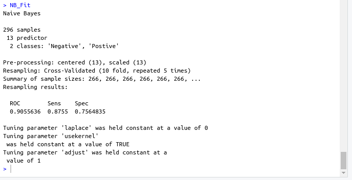
![data](NB.png)
---
# Training using [caret](https://cran.r-project.org/web/packages/caret/index.html)

###2. [Decision tree](https://en.wikipedia.org/wiki/Decision_tree_learning) model
```sh
DT_Fit <- train(
target ~.,
data = data,
method = "rpart",
preProc = c("center","scale"),
tuneLength =15,
trControl = cntrl,
metric = "ROC"
)
```
---
# Training using [caret](https://cran.r-project.org/web/packages/caret/index.html)
###2. [ tree](https://en.wikipedia.org/wiki/Decision_tree_learning) model
###Output screenshot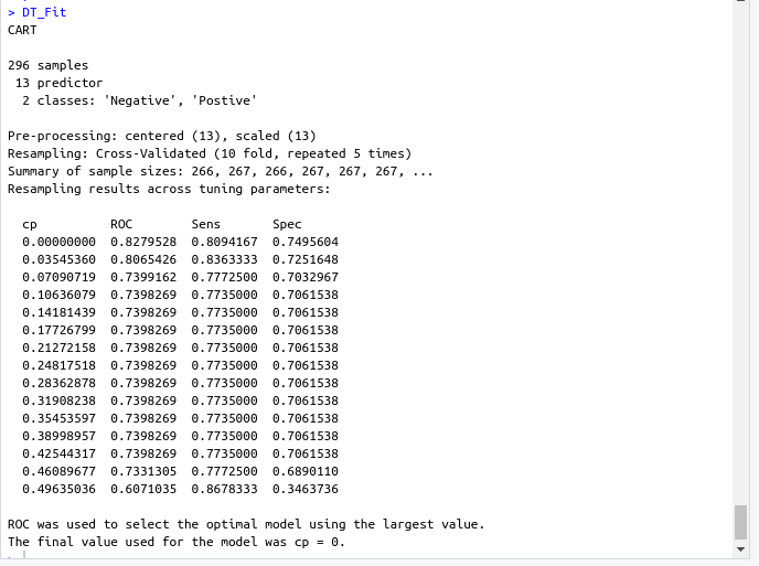
![data](DT.png)
---
# Training using [caret](https://cran.r-project.org/web/packages/caret/index.html)

###2. [Logistic Regression](https://en.wikipedia.org/wiki/Logistic_regression) model
```sh
Log_Fit <- train(
target ~.,
data = data,
method = "glm",
preProc = c("center","scale"),
tuneLength =15,
trControl = cntrl,
metric = "ROC"
)
```
---
# Training using [caret](https://cran.r-project.org/web/packages/caret/index.html)
###2. [Logistic Regression](https://en.wikipedia.org/wiki/Logistic_regression) model
###Output screenshot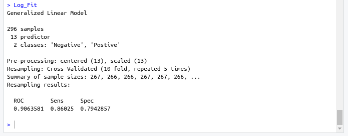
![data](log.png)
---
# Models summary
.left-column[
  ###1. Naïve Bayes model
]  
.right-column[
```remark
-   ROC  : 0.9055636
-   Sens : 0.8755
-   Spec : 0.7564835
```
]
---
# Models summary
.left-column[
  ###1. Naïve Bayes model
  ###2. Decision tree model
]  
.right-column[
```remark
-   ROC  : 0.9055636
-   Sens : 0.8755
-   Spec : 0.7564835
```
```remark
-   ROC  : 0.8279528
-   Sens : 0.8094167
-   Spec : 0.7495604
```
]
---
# Models summary
.left-column[
  ###1. Naïve Bayes model
  ###2. Decision tree model
  ###3. Logistic Regression model
]  
.right-column[
```remark
-   ROC  : 0.9055636
-   Sens : 0.8755
-   Spec : 0.7564835
```
```remark
-   ROC  : 0.8279528
-   Sens : 0.8094167
-   Spec : 0.7495604
```
```remark
-   ROC  : 0.9063581
-   Sens : 0.86025
-   Spec : 0.7942857
```
]
---

class:center,100%
![FilthyFrank](filthyF.jpg)

---
template: inverse
class:center, middle
#Made by
##[Adel Refat](https://adel-elmala.github.io)
---
class:center, middle
#THANKS